Module 5
Module 5
Memory Management
Memory Hierarchy Overview
Computer memory is organized as a hierarchy based on speed, cost, and capacity.
Faster memory is more expensive and smaller; slower memory is cheaper and larger.
General order (fastest → slowest):
Registers → Cache → Main Memory (RAM) → Secondary Storage → Tertiary Storage
CPU Registers
Description
- Small storage locations inside the CPU
- Hold operands, addresses, and intermediate results
Speed
- Fastest memory in the system
- Access time: ~1 CPU cycle (sub-nanosecond)
Cost
- Extremely high cost per bit
- Implemented using flip-flops
Capacity
- Very small (bytes to a few kilobytes per core)
Use Case
- Immediate data required for instruction execution
Cache Memory
Description
- High-speed memory between CPU and RAM
- Stores frequently accessed data
Levels
- L1 Cache: Smallest, fastest
- L2 Cache: Larger, slightly slower
- L3 Cache: Shared, largest, slowest cache
Speed
- L1: ~1–2 ns
- L2: ~3–10 ns
- L3: ~10–20 ns
Cost
- Very high (SRAM-based)
- Cheaper than registers, costlier than RAM
Capacity
- KBs to tens of MBs
Use Case
- Reduce average memory access time
Main Memory (RAM)
Description
- Primary working memory for programs and data
- Volatile (data lost on power-off)
Type
- DRAM (Dynamic RAM)
Speed
- ~50–100 ns access time
Cost
- Moderate cost per bit
- Cheaper than cache, costlier than storage
Capacity
- Typically 4 GB to 128 GB+
Use Case
- Holds active programs and operating system
Secondary Memory (Storage)
Description
- Non-volatile long-term storage
Types
- SSD (Solid State Drive)
- HDD (Hard Disk Drive)
Speed
- SSD: ~50–100 µs
- HDD: ~5–10 ms
Cost
- Low cost per bit
- HDD cheaper than SSD
Capacity
- Hundreds of GBs to multiple TBs
Use Case
- Store OS, applications, and user data
Tertiary / Offline Storage
Description
- Used for backups and archival storage
Examples
- Magnetic tape
- Optical discs
- Cloud cold storage
Speed
- Very slow (seconds to minutes access time)
Cost
- Lowest cost per bit
Capacity
- Very large (TBs to PBs)
Use Case
- Long-term data retention and backups
Comparative Summary
| Memory Type | Speed | Cost per Bit | Capacity |
|---|---|---|---|
| Registers | Fastest | Highest | Very Small |
| Cache | Very Fast | Very High | Small |
| RAM | Fast | Medium | Medium–Large |
| SSD / HDD | Slow | Low | Large |
| Tertiary | Slowest | Lowest | Very Large |
Memory Management is a core function of an Operating System (OS) that handles
the efficient use of primary memory (RAM).
It ensures that:
- Programs get the memory they need
- Memory is used efficiently
- Programs do not interfere with each other
Definition of Memory Management
Memory management refers to the process by which an operating system:
- Allocates memory to processes
- Deallocates memory when no longer needed
- Protects memory from unauthorized access
- Optimizes memory utilization and system performance
Objectives of Memory Management
- Efficient utilization of memory
- Fast access to data and instructions
- Protection and isolation of processes
- Support for multitasking and multiprogramming
- Minimize fragmentation
Memory Allocation
Memory Allocation is the process of assigning memory space to a program or process.
The OS:
- Keeps track of used and free memory blocks
- Allocates memory when a process starts
Types of Allocation
- Contiguous allocation
- Non-contiguous allocation
Memory Deallocation
Memory Deallocation occurs when a process terminates or releases memory.
Importance:
- Prevents memory wastage
- Makes memory available for other processes
- Avoids memory leaks
The OS updates its memory management tables accordingly.
Memory Protection
Memory Protection ensures that one process cannot access another process’s memory.
Methods:
- Base and limit registers
- Protection bits
- Access control mechanisms
Benefits:
- System stability
- Data security
- Error isolation
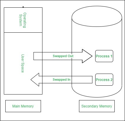
Memory Swapping
Swapping is the process of moving processes between main memory and disk.
- Inactive processes are swapped out to disk
- Active processes are swapped into memory
Purpose:
- Frees physical memory
- Enables execution of more processes
Swapping is a key component of virtual memory.
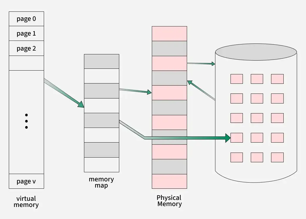
Virtual Memory
Virtual Memory allows programs to use more memory than physically available.
Key features:
- Uses disk as an extension of RAM
- Only required portions of a program are loaded into memory
- Improves multitasking capability
Memory Mapping
Memory Mapping translates virtual addresses to physical addresses.
Performed using:
- Page tables
- Memory Management Unit (MMU)
Advantages:
- Transparent to users
- Efficient memory access
- Supports virtual memory
Memory Fragmentation
Fragmentation occurs when memory is broken into small unusable pieces.
Types:
- Internal Fragmentation
- External Fragmentation
Impact:
- Wastage of memory
- Difficulty in allocating large blocks
Memory Compaction
Memory Compaction is a technique to reduce external fragmentation.
- Moves processes to make free memory contiguous
- Improves memory utilization
- Time-consuming operation
Memory Paging
Paging divides memory into fixed-size units called pages.
Components:
- Pages (virtual memory)
- Frames (physical memory)
- Page table
Benefits:
- Eliminates external fragmentation
- Efficient handling of large memory
Page Table
A Page Table stores the mapping between:
- Virtual page numbers
- Physical frame numbers
Used by: - Memory Management Unit (MMU)
Essential for address translation in paging systems.
Memory Protection
- Memory protection is required to prevent:
- One process from accessing another process’s memory
- User processes from modifying operating system memory
Relocation and Limit Registers
- Protection can be provided using:
- Relocation register
- Limit register
Relocation Register
- Contains:
- The value of the smallest physical address
- Example:
- Relocation register = 100040
Limit Register
- Contains:
- The range of logical addresses
- Example:
- Limit register = 74600
- Logical addresses must be less than the limit value
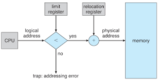
Address Validation
- Every logical address generated by the CPU is:
- Checked against the limit register
- If the logical address exceeds the limit:
- A protection fault occurs
Address Mapping by MMU
- If the logical address is valid:
- The Memory Management Unit (MMU) maps it
- Mapping is done by:
- Adding the logical address to the relocation register
- Mapped (physical) address is sent to memory
Role of MMU
- MMU performs:
- Dynamic address translation
- Ensures:
- Processes access only their allocated memory region
Dispatcher and Context Switch
- When the CPU scheduler selects a process:
- The dispatcher performs a context switch
- During context switch:
- Relocation register is loaded
- Limit register is loaded
- Values correspond to the selected process
Protection Benefits
- Every CPU-generated address is checked
- Ensures protection of:
- Operating system memory
- Other users’ programs and data
- Prevents illegal memory access
Dynamic OS Size Support
- Relocation-register scheme allows:
- Operating system size to change dynamically
- No need to fix OS memory location permanently
Swapping
- Swapping is a memory management technique used by the operating system
- A process must be in memory to be executed
- Swapping allows processes to be temporarily moved out of main memory to disk
Swapping and Priority-Based Scheduling
- A variant of swapping is used in priority-based scheduling algorithms
- If a higher-priority process arrives:
- The OS swaps out a lower-priority process
- Loads and executes the higher-priority process
- After completion:
- The lower-priority process is swapped back in
- Execution resumes from where it stopped
Roll Out and Roll In
- This priority-based swapping technique is called:
- Roll out → swapping a process out of memory
- Roll in → swapping a process back into memory
- Commonly used in systems with limited memory
Memory Space and Swapping
- Normally, a swapped-out process is brought back into:
- The same memory space it previously occupied
- This restriction depends on the address binding method
Address Binding and Swapping
- Assembly-time or Load-time binding
- Physical addresses are fixed
- Process cannot be moved to a different memory location
- Execution-time binding
- Physical addresses computed at runtime
- Process can be swapped into a different memory space
Backing Store
- Swapping requires a backing store
- Usually implemented using a fast disk
- Requirements:
- Large enough to store memory images of all users
- Must support direct access to memory images
Ready Queue and Process States
- The system maintains a ready queue
- Contains processes that are:
- In memory, or
- On the backing store
- All processes in the ready queue are ready to execute
Role of the Dispatcher
- The CPU scheduler selects a process
- The dispatcher checks:
- Whether the selected process is in memory
- If not in memory and no free space exists:
- A process currently in memory is swapped out
- The required process is swapped in
- Registers are reloaded and control is transferred
Context Switch Time in Swapping
- Context-switch time in a swapping system is high
- Dominated by disk I/O operations
- Swap time significantly affects system performance
Swap Time Example (Given Values)
Assumptions:
- Process size: 1 MB
- Disk transfer rate: 5 MB/s
Calculation:
- Transfer time = 1000 KB / 5000 KB per second
- = 1 / 5 second
- = 200 milliseconds
Total Swap Time Calculation
- Average disk latency: 8 milliseconds
- Time for one swap (in or out):
- 200 ms + 8 ms = 208 milliseconds
- Since both swap out and swap in are required:
- Total swap time = 416 milliseconds
Impact on CPU Scheduling
- High swap time reduces CPU efficiency
- For efficient CPU utilization:
- Execution time must be much larger than swap time
Swapping and Round-Robin Scheduling
- In round-robin scheduling:
- Time quantum should be significantly larger than swap time
- Given swap time ≈ 0.416 seconds
- Time quantum must be greater than 0.416 seconds
Contiguous Memory Allocation
- Main memory must accommodate:
- The operating system
- Multiple user processes
- Memory is typically divided into:
- One partition for the resident OS
- One partition for user processes
Placement of the Operating System
- The operating system may be placed in:
- Low memory, or
- High memory
- The major factor affecting this decision:
- Location of the interrupt vector
- Since interrupt vectors are usually in low memory:
- The OS is commonly placed in low memory
Need for Multiprogramming
- Multiple user processes should reside in memory simultaneously
- This improves CPU utilization
- Memory must be allocated to processes waiting in the input queue
Contiguous Memory Allocation Concept
- Each process is allocated:
- A single contiguous block of memory
- A process must fit entirely within one memory region
Fixed-Size Partitioning
- One of the simplest memory allocation techniques
- Memory is divided into:
- Several fixed-size partitions
- Each partition can hold:
- Exactly one process
- Degree of multiprogramming:
- Limited by the number of partitions
Multiple-Partition Method
- When a partition is free:
- A process from the input queue is loaded into it
- When a process terminates:
- The partition becomes available for reuse
- The OS maintains:
- A table of free and occupied memory partitions
Process Life Cycle in Memory
- Processes enter the system and wait in an input queue
- When memory is allocated:
- Process is loaded into memory
- Process competes for CPU time
- When a process terminates:
- Memory is released
- Space can be reassigned to another process
Dynamic Memory and Holes
- Free memory areas are called holes
- Holes vary in size and are scattered throughout memory
- When a process arrives:
- The OS searches for a hole large enough
Hole Splitting
- If a hole is larger than required:
- It is split into two parts:
- One allocated to the process
- One returned to the set of holes
- It is split into two parts:
Hole Merging
- When a process releases memory:
- The block becomes a new hole
- If adjacent holes exist:
- They are merged into one larger hole
Dynamic Storage Allocation Problem
- The problem of:
- Satisfying a request of size n
- From a list of free holes
- This is known as:
- Dynamic storage allocation
Memory Allocation Strategies
- The OS selects an appropriate hole using:
- First Fit
- Best Fit
- Worst Fit
First Fit Strategy
- Allocates:
- The first hole that is large enough
- Search may begin:
- From the beginning of the hole list, or
- From where the last search ended
- Search stops once a suitable hole is found
- Generally faster than other methods
Best Fit Strategy
- Allocates:
- The smallest hole that is large enough
- Requires:
- Searching the entire list (unless sorted by size)
- Produces:
- The smallest leftover hole
Worst Fit Strategy
- Allocates:
- The largest available hole
- Requires:
- Searching the entire list (unless sorted)
- Produces:
- The largest leftover hole
Comparison of Fit Strategies
- Simulations show:
- First fit and best fit outperform worst fit
- In terms of storage utilization:
- First fit ≈ Best fit
- In terms of speed:
- First fit is generally faster
Fragmentation
- Memory fragmentation occurs when memory is wasted or inefficiently used
- Fragmentation can be:
- Internal fragmentation
- External fragmentation
External Fragmentation
- External fragmentation exists when:
- Enough total memory is available
- Memory is not contiguous
- Free memory is broken into:
- Many small holes
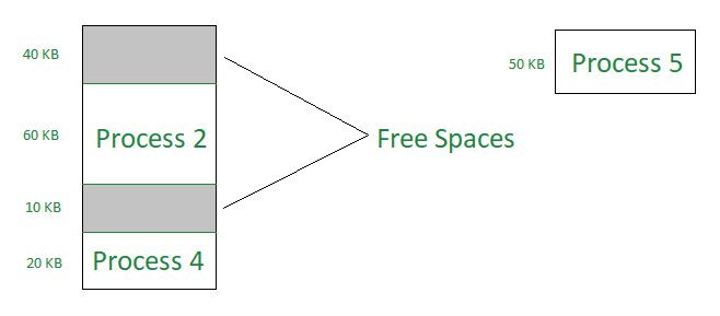
Worst-Case External Fragmentation
- In the worst case:
- A small free block exists between every two processes
- Although total free memory is sufficient:
- It cannot be used effectively
- If all free memory were in one block:
- Several more processes could be executed
Compaction
- Compaction is a solution to external fragmentation
- Goal:
- Shuffle memory contents
- Combine all free memory into one large block
Conditions for Compaction
- Compaction is not always possible
- If relocation is:
- Static (assembly-time or load-time)
- Compaction cannot be done
- Dynamic (execution-time)
- Compaction is possible
- Static (assembly-time or load-time)
Dynamic Relocation and Compaction
- With dynamic relocation:
- Programs and data are moved in memory
- Base (relocation) register is updated
- No need to change logical addresses in the program
Cost of Compaction
- Cost of compaction must be considered
- Simplest compaction algorithm:
- Move all processes toward one end of memory
- Move all holes toward the other end
- Result:
- One large free memory block
- Drawback:
- Can be expensive in time and overhead
Noncontiguous Memory Allocation
- Another solution to external fragmentation:
- Allow a process’s logical address space to be noncontiguous
- Physical memory can be allocated:
- Wherever space is available
Paging and Segmentation
- Two complementary techniques support noncontiguous allocation:
- Paging
- Segmentation
- Paging and segmentation:
- Reduce or eliminate external fragmentation
- Can be used together
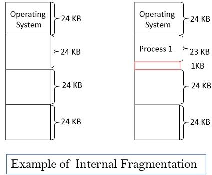
Internal Fragmentation
- Internal fragmentation occurs when:
- Allocated memory is slightly larger than requested
- The unused portion:
- Lies inside the allocated partition
- Cannot be used by other processes
- This unused space is called internal fragmentation
Example of Internal Fragmentation
- Consider a multiple-partition allocation scheme
- Available hole size: 18,464 bytes
- Process requests: 18,462 bytes
- If allocated exactly:
- Remaining hole = 2 bytes
- Problem:
- Overhead of managing a 2-byte hole is greater than the hole itself
Solution Approach
- Physical memory is divided into:
- Fixed-sized blocks
- Memory is allocated in:
- Units of block size
- This approach:
- Simplifies allocation
- Accepts some internal fragmentation to avoid excessive overhead
Virtual Memory
- Virtual memory is a memory management technique that allows a computer to:
- Use more memory than is physically available (RAM)
- When RAM is full:
- Data is temporarily transferred to a hard drive or SSD
- This frees up RAM for active processes
- Data moved to storage can be retrieved when needed
- Managed entirely by the operating system
- Transparent to applications:
- Programs behave as if full physical memory is available
- Advantages:
- Allows more programs to run simultaneously
- Supports larger data sets
- Limitations:
- Disk access is slower than RAM
- Excessive virtual memory use can cause:
- Slow performance
- System unresponsiveness
- Heavy usage may fragment the disk, degrading performance further
Paging
- Paging is a memory-management scheme that allows:
- The physical address space of a process to be noncontiguous
- Eliminates the need to fit variable-sized memory chunks into contiguous space
- Due to its advantages:
- Paging is commonly used in modern operating systems
Hardware Support for Paging
- Paging is supported directly by hardware
- Implemented on:
- 64-bit microprocessors
- Hardware assistance makes paging efficient and practical
Memory Division in Paging
- Physical memory is divided into:
- Fixed-sized blocks called frames
- Logical (virtual) memory is divided into:
- Fixed-sized blocks of the same size called pages
Loading Pages into Memory
- When a process is executed:
- Its pages are loaded from the backing store
- Pages can be placed into any available memory frames
- Contiguous allocation is not required
Backing Store Structure
- The backing store is divided into:
- Fixed-sized blocks
- These blocks are:
- The same size as memory frames
- This simplifies paging operations
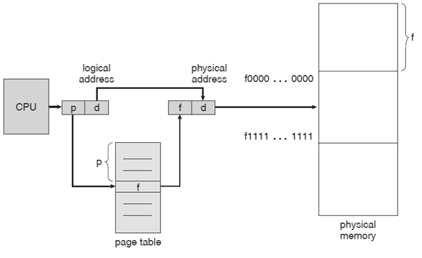
Address Structure in Paging
- Every CPU-generated address is divided into:
- Page number (p)
- Page offset (d)
- The page number is used to:
- Index into the page table
Page Table
- The page table stores:
- Base address of each page in physical memory
- Each entry maps:
- A page number to a frame number

Address Translation
- The physical address is formed by:
- Combining the frame base address (from page table)
- With the page offset
- This physical address is sent to:
- The memory unit
- Page size is typically a power of 2
- Common page sizes range from:
- 512 bytes to 16 MB
- Most modern systems use:
- 4 KB to 8 KB pages
- Some systems support even larger page sizes
Logical Address Structure
- If logical address space size = 2^m
- Page size = 2^n addressing units (bytes or words)
- Then:
- High-order (m − n) bits → page number (p)
- Low-order n bits → page offset (d)
Logical Address Representation
- Logical address format:
- < p , d >
- Where:
- p = index into the page table
- d = displacement within the page
Fragmentation in Paging
- Paging eliminates external fragmentation
- Any free frame can be allocated to any process
- Contiguous memory is not required
Internal Fragmentation in Paging
- Paging may cause internal fragmentation
- Occurs when:
- Process size does not align with page boundaries
- The last frame may not be completely used
Internal Fragmentation Example
- Page size: 2,048 bytes
- Process size: 72,766 bytes
- Pages required:
- 35 full pages + 1,086 bytes
- Frames allocated:
- 36 frames
- Internal fragmentation:
- 2,048 − 1,086 = 962 bytes
Hardware Support for Paging
- Hardware support is required to implement page tables efficiently
- Page-table implementation can be done in several ways
Page Table Using Registers
- Simplest implementation:
- Page table stored in dedicated registers
- CPU dispatcher:
- Reloads these registers during a context switch
- Suitable when:
- Page table is reasonably small
- Example: 256 entries
- Advantage:
- Very fast access
Large Page Tables in Modern Systems
- Contemporary systems support:
- Very large page tables
- Example: up to 1 million entries
- Using registers for such large tables:
- Not feasible
Page Table in Main Memory
- Page table is stored in:
- Main memory
- A special register called:
- Page-Table Base Register (PTBR)
- Points to the page table
- Changing the page table:
- Requires changing only the PTBR
Problem with PTBR Approach
- Accessing a memory location requires:
- Accessing the page table using PTBR
- Accessing the actual memory location
- This results in:
- Two memory accesses per reference
- Leads to slower memory access time
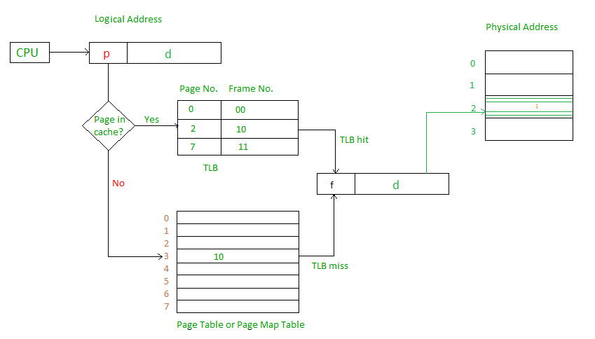
Translation Look-Aside Buffer (TLB)
- Standard solution to reduce memory access time:
- Translation Look-Aside Buffer (TLB)
- TLB is:
- Small
- Fast
- Hardware cache
Characteristics of TLB
- TLB is:
- Associative, high-speed memory
- Each TLB entry contains:
- Key (tag) – page number
- Value – frame number
TLB Operation
- When an address is presented:
- It is compared with all TLB keys simultaneously
- If a match is found:
- Corresponding frame number is returned
- Search operation:
- Very fast
- Hardware cost:
- High
TLB Size
- Number of TLB entries is limited
- Typical size:
- 64 to 1,024 entries
- Small size balances:
- Speed
- Hardware cost
Segmentation
- Segmentation is a memory management technique
- Memory is divided into variable-sized segments
- Each segment corresponds to a logical unit of a program
- Examples of segments:
- Code segment
- Stack
- Heap
- Data structures
Purpose of Segmentation
- Allows dynamic memory allocation at runtime
- Memory need not be allocated entirely at compile time
- Helps:
- Reduce memory wastage
- Improve utilization of available memory
- Matches programmer’s logical view of memory
Segmented Memory System
- Each segment is assigned:
- A Segment Identifier (SID)
- A base address
- Base address:
- Indicates the first byte of the segment in physical memory
Memory Allocation in Segmentation
- When a program requests memory:
- OS allocates a segment of required size
- Assigns a unique SID
- Returns the base address to the program
- Segments can be allocated and deallocated dynamically
Addressing in Segmentation
- Programs use relative addressing
- Address of a byte is calculated:
- Relative to the base address of its segment
- Program does not need to know:
- Absolute physical memory addresses
- Supports relocation during execution
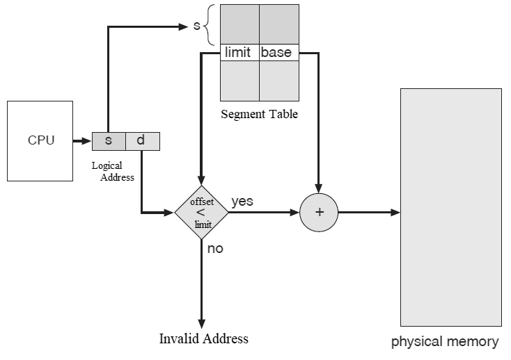
Logical Address Structure
- A logical address has two parts:
- Segment number (s)
- Offset within the segment (d)
- Format:
< s , d >
Segment Table
- Segment number s is used as an index into the segment table
- Each segment table entry contains:
- Base address of the segment
- Limit (length) of the segment
Address Validation and Mapping
- Offset d must satisfy:
0 ≤ d < segment limit
- If valid:
- Physical address = segment base + offset
- If invalid:
- Trap to the operating system
Example: Segment Mapping
- Five segments numbered 0 to 4
- Segment table contains base and limit for each segment
Example Calculations
- Segment 2:
- Base = 4300
- Length = 400 bytes
- Reference to byte 53:
- Physical address = 4300 + 53 = 4353
More Examples
- Segment 3:
- Base = 3200
- Reference to byte 852:
- Physical address = 3200 + 852 = 4052
Protection Example
- Segment 0:
- Length = 1000 bytes
- Reference to byte 1222:
- Offset exceeds segment limit
- Results in a trap to the operating system
Variable Partition Memory Allocation
- Variable partition memory allocation is a memory management technique
- Main memory is divided into variable-sized partitions
- Partitions are created dynamically based on program requirements
- Memory is allocated to programs as needed
Characteristics of Variable Partitioning
- Partition sizes are not fixed
- Better utilization of memory compared to fixed partitions
- Can lead to fragmentation
- Commonly used allocation strategies determine efficiency
Page Fault
- A page fault is an exception that occurs when:
- A program tries to access a page
- That page is not present in physical memory
- The required page is outside the current working set
Page Fault in Virtual Memory
- Virtual memory allows programs to:
- Use more memory than physically available
- Pages are:
- Swapped in and out of physical memory as needed
- When a required page is not in memory:
- A page fault occurs
Page Fault Handling
- On a page fault, the operating system:
- Checks whether the page is in physical memory
- If the page is not present:
- OS selects a page to evict using a page replacement algorithm
- Frees space for the required page
Page Swapping Process
- The requested page is:
- Loaded from secondary storage (disk/SSD)
- This process is called:
- Page swapping or page fault handling
- Once loaded:
- Program execution resumes normally
Performance Impact
- Page faults degrade performance because:
- Disk access is much slower than RAM access
- Excessive page faults can:
- Slow down programs
- Reduce system responsiveness
Importance of Reducing Page Faults
- Minimizing page faults is a key goal of:
- Operating system design
- Memory management strategies
- Efficient page replacement improves:
- System performance
- User experience
Page Replacement Algorithms
- First In First Out (FIFO) – Replaces the page that has been in memory the longest.
- Least Recently Used (LRU) – Replaces the page that has not been used for the longest time.
- Optimal Page Replacement – Replaces the page that will not be used for the longest period in the future.
First-In-First-Out (FIFO) Page Replacement
- FIFO is a basic page replacement algorithm used in operating systems
- It follows the principle:
- The page that was first brought into memory is the first to be replaced
- Replacement occurs when:
- A page fault happens
- No free page frame is available
FIFO Working and Limitation
- The OS maintains:
- A queue of page frames for a process
- New pages are:
- Added to the end of the queue
- When frames are full:
- The page at the front of the queue is replaced
- Advantages:
- Simple
- Easy to implement
- Limitation:
- Suffers from Belady’s Anomaly
- Increasing page frames may increase page faults
Least Recently Used (LRU) Page Replacement Algorithm
- LRU is a widely used page replacement algorithm
- It replaces the page that has been least recently used
- When a page fault occurs:
- The OS must select a page in memory for replacement
- LRU assumes:
- Pages used recently are likely to be used again soon
Working, Advantages, and Limitations of LRU
- OS maintains a list of pages currently in memory
- On every page access:
- The page is moved to the front of the list
- Page replacement:
- The page at the back of the list (least recently used) is removed
- Advantages:
- Keeps frequently used pages in memory
- Performs well in practice
- Limitations:
- Expensive to implement in hardware
- Requires updating the list on every access
- May perform poorly for programs with large, rapid data access
- Improvements:
- Modified versions like Clock or Second Chance algorithms are used
Optimal Page Replacement Algorithm
- Optimal Page Replacement is an ideal page replacement algorithm
- It replaces the page that will not be used for the longest time in the future
- Requires knowledge of future page references
- Not practical for real operating systems
Purpose and Working of Optimal Algorithm
- Used as a theoretical upper bound for comparison
- Other algorithms are evaluated by comparing their page faults with optimal
- Implementation (simulation):
- Scan the entire page reference sequence
- For each page, determine time until next use
- Replace the page with the maximum future use time
- If a page is never referenced again, use end of sequence as reference
- Useful for:
- Performance analysis
- Benchmarking page replacement algorithms
Disk Structure
- Disk structure defines how data is organized and stored on a storage device
- Determines how data is stored, accessed, and protected
- Essential for efficient data management and system performance
File System
- Most common disk structure
- Organizes data into files and directories (folders)
- Manages:
- Disk space allocation
- File locations
- Access permissions
- Enables operating systems and applications to access data
Types of File Systems
- Different operating systems use different file systems:
- NTFS – Windows
- HFS+ – macOS
- ext4 – Linux
- Some file systems are designed for specific uses
- Example: FAT for removable storage devices
Disk Partitions
- Disk can be divided into multiple partitions
- Partition tables define:
- Size of each partition
- Location on disk
- Each partition can have its own file system
Boot Records and Importance
- Boot records store information needed to start the operating system
- Loaded when the computer powers on
- Disk structures ensure:
- Proper system startup
- Data reliability
- Protection against data corruption

| Category | Details |
|---|---|
| Platter Size (Historical Range) | 0.85” to 14” |
| Common Platter Sizes | 3.5”, 2.5”, 1.8” |
| Storage Capacity | 30 GB to 3 TB per drive |
| Theoretical Transfer Rate | 6 Gb/sec |
| Effective Transfer Rate | ~1 Gb/sec |
| Seek Time Range | 3 ms to 12 ms |
| Typical Desktop Seek Time | ~9 ms |
|---|---|
| Average Seek Time Basis | Measured or calculated using 1/3 of total tracks |
| Latency Dependency | Based on spindle (RPM) speed |
| Latency Formula | Latency = 60 / RPM |
| Average Latency | ½ × (60 / RPM) |
Disk Addressing and Logical Block Mapping
- Disk drives are addressed as large 1-dimensional arrays of logical blocks
- A logical block is the smallest unit of data transfer
- Low-level formatting creates logical blocks on the physical disk
- Logical blocks are mapped sequentially to disk sectors
- Sector 0 is the first sector of the first track on the outermost cylinder
- Mapping proceeds:
- Through the current track
- Then remaining tracks of the same cylinder
- Then inward cylinder by cylinder
- Logical-to-physical address mapping is generally simple
- Bad sectors complicate address mapping
- Number of sectors per track may be non-constant due to constant angular velocity (CAV)
Disk Scheduling
- The operating system is responsible for using disk hardware efficiently
- Main goals:
- Fast access time
- High disk bandwidth
- Disk scheduling focuses on minimizing seek time
- Seek time is approximately proportional to seek distance
Disk I/O Requests and Bandwidth
- Disk bandwidth = total bytes transferred ÷ total time from first request to last completion
- Disk I/O requests can originate from:
- Operating system
- System processes
- User processes
- Each I/O request includes:
- Input or output mode
- Disk address
- Memory address
- Number of sectors to transfer
Request Queues and Scheduling Need
- The OS maintains a queue of disk I/O requests for each disk or device
- If the disk is idle, it can immediately service a request
- If the disk is busy, new requests are queued
- Disk scheduling and optimization algorithms are meaningful only when a request queue exists
Rotational Latency
- Rotational latency is the delay experienced while the disk rotates to position the read/write head over the desired sector
- The read/write head must wait for the correct sector to pass underneath
- Determined by disk rotational speed (RPM)
- Important factor in HDD performance and data access time
Rotational Latency – Calculation and Optimization
- Average rotational latency = ½ × time for one full disk rotation
- Total access time = Average seek time + Average rotational latency
- Reducing rotational latency improves performance:
- Increase rotational speed
- Use disks with larger capacity
- Use SSDs, which eliminate rotational latency
Seek Time
- Seek time is the time required for a hard disk's read/write head to move to the track containing the desired data
- Measures how quickly the head can position itself over the correct location on the disk
- Critical factor in disk performance and access speed
Seek Time – Measurement and Importance
- Typically measured in milliseconds (ms)
- Lower seek times are better for faster data retrieval
- Varies depending on hard drive model and design
- Directly affects the efficiency of data access and transfer
Rotational Latency & Seek Time – Numerical Example
- To calculate rotational latency and seek time, you need:
- Rotational speed of the disk (RPM)
- Average seek time (ms)
- Distance the read/write head moves (tracks)
Example Hard Disk Specifications
- Rotational speed: 7200 RPM
- Average seek time: 8 ms
- Distance to move read/write head: 3 tracks
- Total tracks on disk: 16,384
Rotational Latency Calculation
- Formula:
Rotational latency = 60 / (RPM × 2) ms - Calculation:
Rotational latency = 7200 / 60 / 2 = 60 / 2 = 30 ms - Result: Rotational latency = 30 ms
Seek Time Calculation
- Formula:
Seek time = Average seek time × (Tracks moved / Total tracks) - Calculation:
Seek time = 8 × (3 / 16384) = 0.0147 ms - Result: Seek time = 0.0147 ms
Scheduling algorithms
- FIFO - First come first served
- SSTF - Shortest seek time first
- SCAN
- C-SCAN
- C-LOOK
Refer: os.surajgowda.in/disk-scheduling for simulation
Disk Management
- Disk Management is a utility tool in Windows for managing storage devices
- Allows users to view partitions and volumes
- Enables creation, formatting, deletion, and assignment of drive letters
Disk Management – Partition Operations
- Users can extend, shrink, or move partitions
- Helps optimize disk space and manage storage efficiently
- Supports conversion between disk types: Basic ↔ Dynamic
Disk Management – Advanced Features
- Configure advanced settings:
- Mirrored volumes
- RAID arrays
- Useful for managing multiple storage devices
- Enhances disk performance and organization
RAID – Redundant Array of Independent Disks
- RAID = Redundant Array of Inexpensive Disks
- Uses multiple disk drives to provide reliability via redundancy
- Increases mean time to failure (MTTF) of storage system
Reliability Factors in RAID
- Mean Time to Repair (MTTR): exposure time when another failure could cause data loss
- Mean Time to Data Loss (MTDL): depends on MTTF and MTTR
- Example:
- Disk MTTF = 1,300,000 hours
- MTTR = 10 hours
- MTDL = 100,000² / (2 × 10) = 500 × 10⁶ hours ≈ 57,000 years
RAID – Performance & Improvements
- Often combined with NVRAM to improve write performance
- Multiple disks can work cooperatively for better efficiency
- Enhances reliability, performance, and fault tolerance
Disk Striping and RAID Levels
- Disk striping: uses a group of disks as a single storage unit
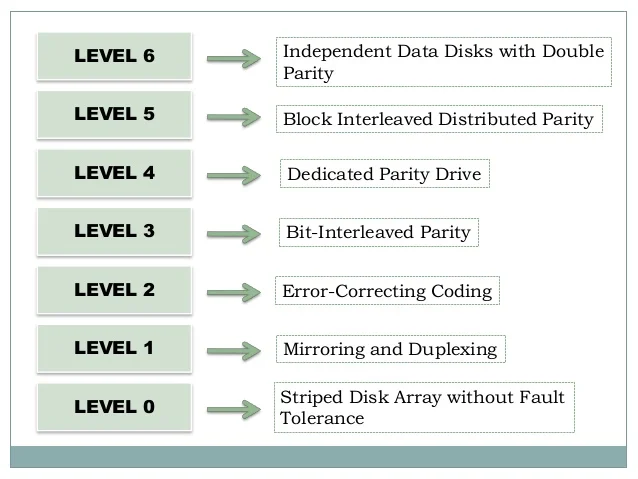
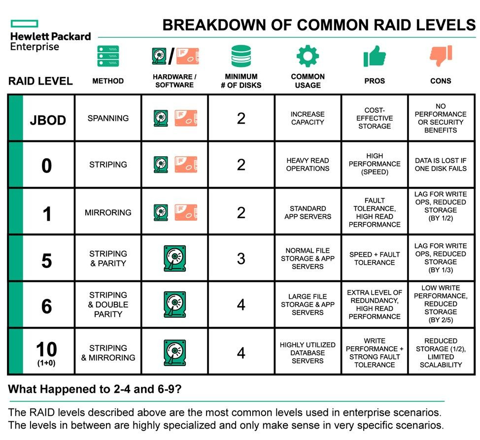
- RAID is organized into six different levels
- Improves both performance and reliability through redundancy
RAID Mirroring and Stripes
- RAID 1 – Mirroring/Shadowing: keeps a duplicate of each disk
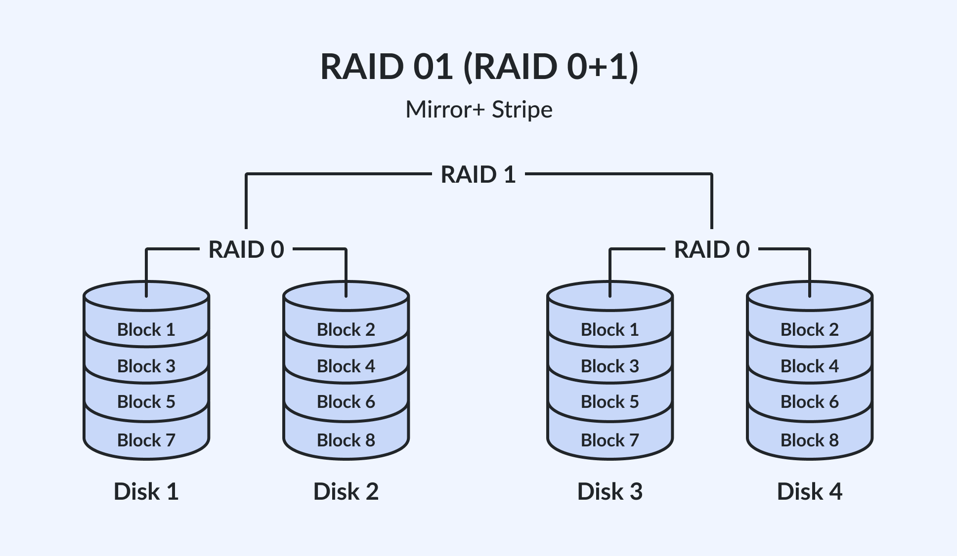
- RAID 1+0 (Striped Mirrors) / 0+1 (Mirrored Stripes): combines high performance and high reliability
- RAID 4, 5, 6 – Block Interleaved Parity: provides redundancy with less storage overhead
RAID Array Management
- RAID within a single array can still fail if the array fails
- Automatic replication between arrays is common for added safety
- Hot-spare disks: unallocated disks that replace failed disks automatically and rebuild data
RAID levels